Charge Sign Identification Improvement in the Tracker Analysis
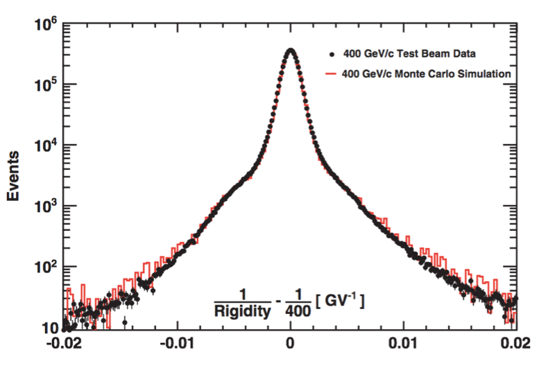
Test beam data are crucial in understanding the detector performance details. Figure 1 shows the comparison between data and the Monte Carlo simulation of the inverse rigidity measured by the tracker for 400 GeV/c test beam protons. As seen, the Monte Carlo simulation describes not only detector resolution effects (the central part of the distribution) but also the various interactions with the detector materials including multiple, large angle, elastic, and quasi-elastic scattering (tails of the distribution). Figure 1 shows that the agreement between the data and the Monte Carlo simulation extends over five orders of magnitude.
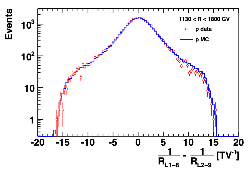
Extensive verification of the detector performance at the energies at and above 1 TeV were performed as part of the current analysis. To study the tracker performance beyond the test beam momentum (400 GeV/c proton beam), we used the Space Station data to compare the rigidity measured using the upper layers of the tracker with the rigidity measured with the lower layers. Figure 2 shows that the difference of these inverse rigidities is centered at zero and in good agreement with the Monte Carlo simulation for the rigidity range [1130 - 1800] GV, that is close to the Maximal Detectable Rigidity, MDR, of 2 TV for $|Z|=1$ particles.
The improvements in the Monte Carlo simulation, based on the results of additional extensive calibrations in space, provide an accurate description of the data up to multi-TeV energies.
Charge confusion is a critical parameter of the spectrometer, which allows to distinguish negatively charged cosmic rays from positively charged cosmic rays.
For improvement of the charge sign identification it is important to distinguish positrons from charge-confusion electrons, i.e. those electrons reconstructed with the positive charge sign due to the finite tracker resolution or interactions in the detector materials. To this end a charge confusion estimator $\Lambda_{CC}^{e}$ is defined using the Boosted Decision Trees technique. The estimator combines several measurements: the ratio of the energy from the calorimeter to the momentum from the tracker, $E/p$, the track χ2/d.o.f., momenta reconstructed with different combinations of tracker layers, the number of hits in the vicinity of the track, and the charge measurements in the TOF and in the tracker. With this method, positrons, which have
The charge confusion in data is obtained using the template fitting technique. From the fit to the positive rigidity sample, we obtain the number of positron $N_{e^+}$ events, charge confusion electron background $N_{e^-}^{C.C.}$ events, and proton background events. From the fit to the negative rigidity sample, we obtain the number of electron $N_{e^-}$ events, charge confusion positron background $N_{e^+}^{C.C.}$
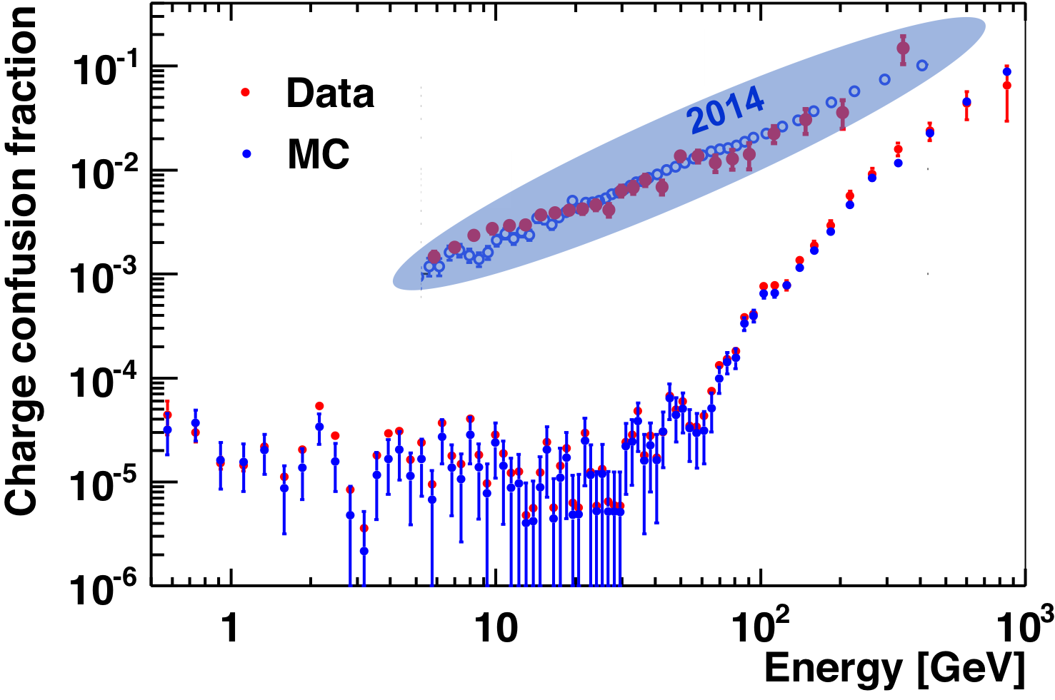
The charge confusion in Monte Carlo simulation is directly calculated as the fraction of electrons being reconstructed with positive rigidity after the same selection cuts as used in data are applied. As an illustration, the comparison between the electron charge confusion fraction in the data and in the Monte Carlo simulation is presented in Figure 3. As seen, the charge confusion is reproduced by the Monte Carlo simulation. In 2014 the charge confusion fraction at 500 GeV was 10%, and now it has been improved to better than 3%.
Similar methods are used to differentiate antiprotons and anti-deuterons from large proton and deuteron backgrounds.