New Reconstruction Method in the Electromagnetic Calorimeter (ECAL) Analysis
The key detector for measurements of electrons and positrons in AMS is the Electromagnetic Calorimeter, ECAL (see Figure 1). The ECAL consists of a multilayer sandwich of lead foils and ∼50,000 scintillating fibers with an active area of 648 × 648 mm2 and a thickness of 166.5 mm, corresponding to 17 radiation lengths, $X_0$. The calorimeter is composed of 9 superlayers, each 18.5 mm thick and made of 11 grooved, 1 mm thick lead foils interleaved with 10 layers of 1 mm diameter scintillating fibers. In each superlayer, the fibers run in one direction only. The 3D imaging capability of the detector is obtained by stacking alternate superlayers with fibers parallel to the ? and ? axes (5 and 4 superlayers, respectively).
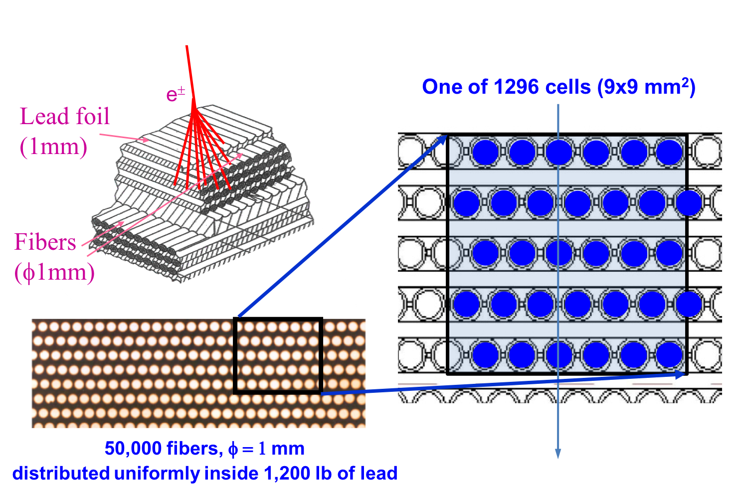
All fibers are read out on one end only by 324 photomultipliers (PMT). Each PMT has four anodes and is surrounded by a magnetic shield which contains light guides, the PMT base and the frontend electronics. Each anode covers an active area of 9 × 9 mm2, corresponding to about 35 fibers, defined as a cell. Figure 1 (left) schematically shows the construction and the optical face of one superlayer of the lead-fiber matrix, against which a grid of PMTs is mounted. These PMT grids on the four ECAL faces define the ECAL coordinate system. Figure 1 (right) illustrates the locations of optical fibers within a cell. In total there are 1296 cells segmented into 18 layers longitudinally, two per superlayer, with 72 transverse cells in each layer providing a fine granularity sampling of the shower in three dimensions. The signals are processed over a wide dynamic range, from a minimum ionizing particle, which produces about 10 photoelectrons per cell, up to the 60,000 photoelectrons produced in one cell by the core of the electromagnetic shower of a 1 TeV electron, corresponding to deposited energy of 60 GeV.
Reconstruction of electrons and positrons in the calorimeter uses a 3-dimensional shower parametrization, which accounts for the detector specifics: finite size of the calorimeter, non-uniform efficiency of the signal collection, and saturation effects due to the electronics and due to high energy density in the active calorimeter elements (A. Kounine, Z. Weng, W. Xu, and C. Zhang, Nucl. Instr. Methods Sect. A, 869 110 (2017)).
An individual electromagnetic shower is described by seven parameters, which fully determine the observed pattern of energy depositions in the calorimeter cells: the shower energy ($E_0$); the 3-dimensional spatial point, ($x_0$ , $y_0$ , $z_0$ ), corresponding to the location of the shower maximum in the ECAL coordinate system; the two angles ($K_X$, $K_Y$) that, together with the spatial point, define the shower axis; and the location ($T_0$) of the shower maximum on the shower axis. The parameter ($\beta$) depends on the specific construction and materials of the calorimeter. This is a minimal parameter set, which allows accurate shower parametrization of individual showers without introducing noticeable correlation between these parameters.
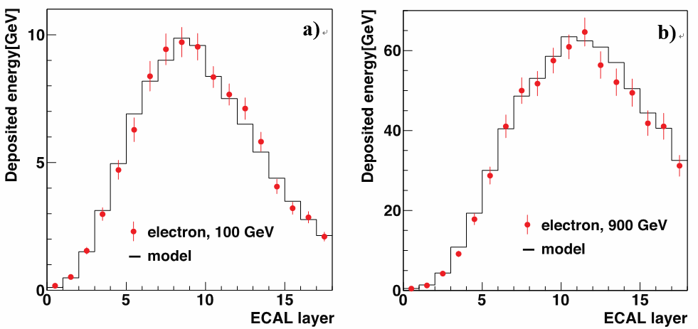
The longitudinal shower profile in terms of the depth t in the calorimeter (in units of radiation length) is described by empirical parametrization [Particle Data Group, Phys. Rev. D 98, 030001 (2018)]:
$$ \frac {dE}{dt}(t) = E_{0} \frac{(\beta t)^{\beta T_{0}}\beta e^{-\beta t}}{\Gamma(\beta T_{0}+1)} $$
using the parameters described above. In our calorimeter, we found that the scale parameter $\beta$ is constant ($\beta=0.65$). The individual shower parameters $E_0$ and $T_0$ are obtained from a fit to observed energy depositions in the ECAL cells of each shower. Figure 2 shows the description of electron showers over a wide energy range.