Improvements in the proton rejection using ECAL
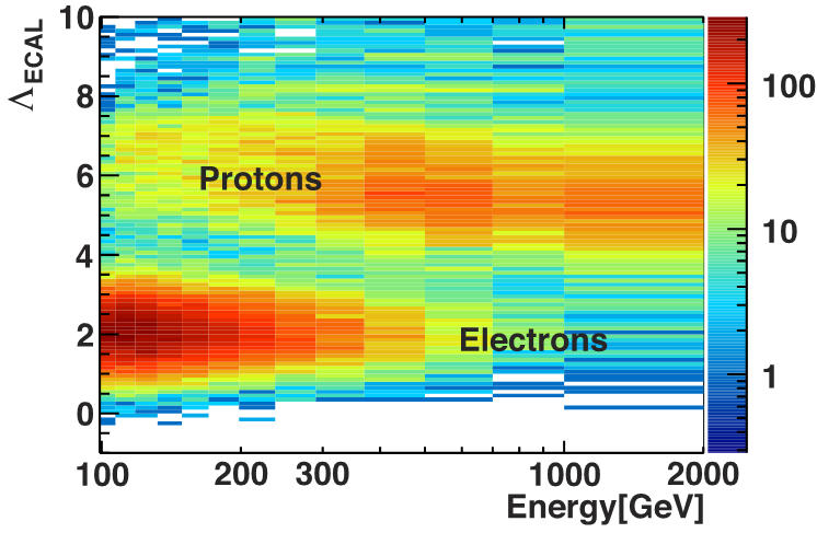
We have improved the identification of electrons and positrons in the TeV energy range. This is achieved by increasing the proton rejection with an ECAL estimator $\Lambda_\text{ECAL}$. The estimator is constructed based on the information from the new ECAL reconstruction described above. It includes variables, which measure the compatibility of energy depositions in the calorimeter cells with that of an electromagnetic shower. It also includes variables that measure the consistency of the shower parameter values (like $z_0$ and $T_0$) with those expected for an electromagnetic shower of energy $E_0$. Altogether there are 16 variables included in the definition of $\Lambda_\text{ECAL}$. The dependence of $\Lambda_\text{ECAL}$ on energy for electrons and protons is shown in Figure 1.
The proton rejection power is evaluated as a function of rigidity as shown in Figure 2. It is significantly improved compared to the traditional method. The improvement is about 20% below 400 GeV and increases to a factor of 5 at 1 TeV. With this new technique the AMS energy reach for cosmic ray positrons and electrons is extended to 2 TeV and beyond.
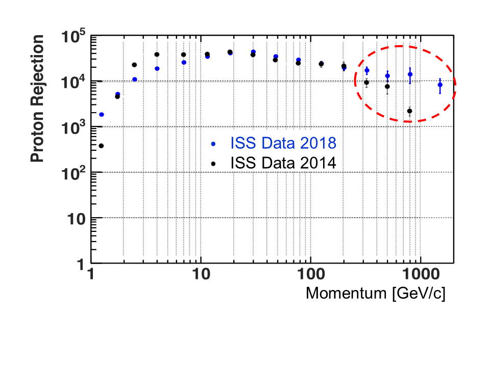
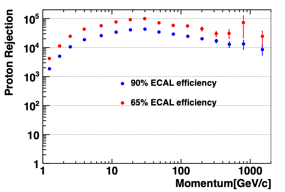
Figure 3 shows that with the new method the proton rejection can be further increased at the highest energies by a factor of three with the tighter $\Lambda_\text{ECAL}$ cut. With the tighter $\Lambda_\text{ECAL}$ cut the electron and positron selection efficiency is reduced from the nominal 90% to 65%.
The fit using $\Lambda_{\rm ECAL}$ templates has been performed in the electron flux analysis to determine the number of electron signal events. In this analysis, events are required to start showers in the first layers of the ECAL. Figure 4 shows the fit results in the energy bins [290, 370], [370, 500], [500, 700], and [700, 1000] GeV. In these energy bins the $\Lambda_{\rm ECAL}$ distribution for antiprotons and charge confusion protons is found to be the same as for ordinary protons. Therefore, to reduce the statistical fluctuation, the charge confusion proton template is constructed using proton data. This is done for each energy bin by selecting protons with the TRD and the tracker, and also requiring the ratio of the ECAL energy and the tracker rigidity $E/|R| < 1.0$. The $\Lambda_{\rm ECAL}$ electron template is energy independent as seen in Figure 4, therefore, the electron signal template is constructed using electron data selected by the TRD and the tracker in the energy range [100 – 1000] GeV to reduce the statistical fluctuation of the template. The shape of the charge confusion positron $\Lambda_{\rm ECAL}$ template is the same as for the electron signal. The amount of the charge confusion positron background is estimated from the Monte Carlo simulation. It amounts to <3% of the electron signal for all these energy bins. As seen in Figure 4, the $\Lambda_{\rm ECAL}$ estimator allows to separate the electron signal from charge confusion proton background to multi-TeV region.
![The projections onto the ?ECAL axis for the different energy bins: (a) [290, 370], (b) [370, 500], (c) [500, 700], and (d) [700, 1000] GeV for the negative rigidity events.](/sites/default/files/inline-images/ecal_proton_rejection.Fig4all.png)