Improvements in the Charge Resolution
The nine tracker layers independently measure the charge $|Z|$ of cosmic rays. The ionization energy losses deposited in the silicon, see Figure 1, are proportional to $Z^{2}$ and this is measured with both the x- and y- side strips.
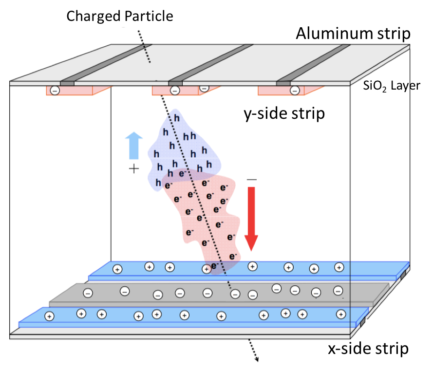
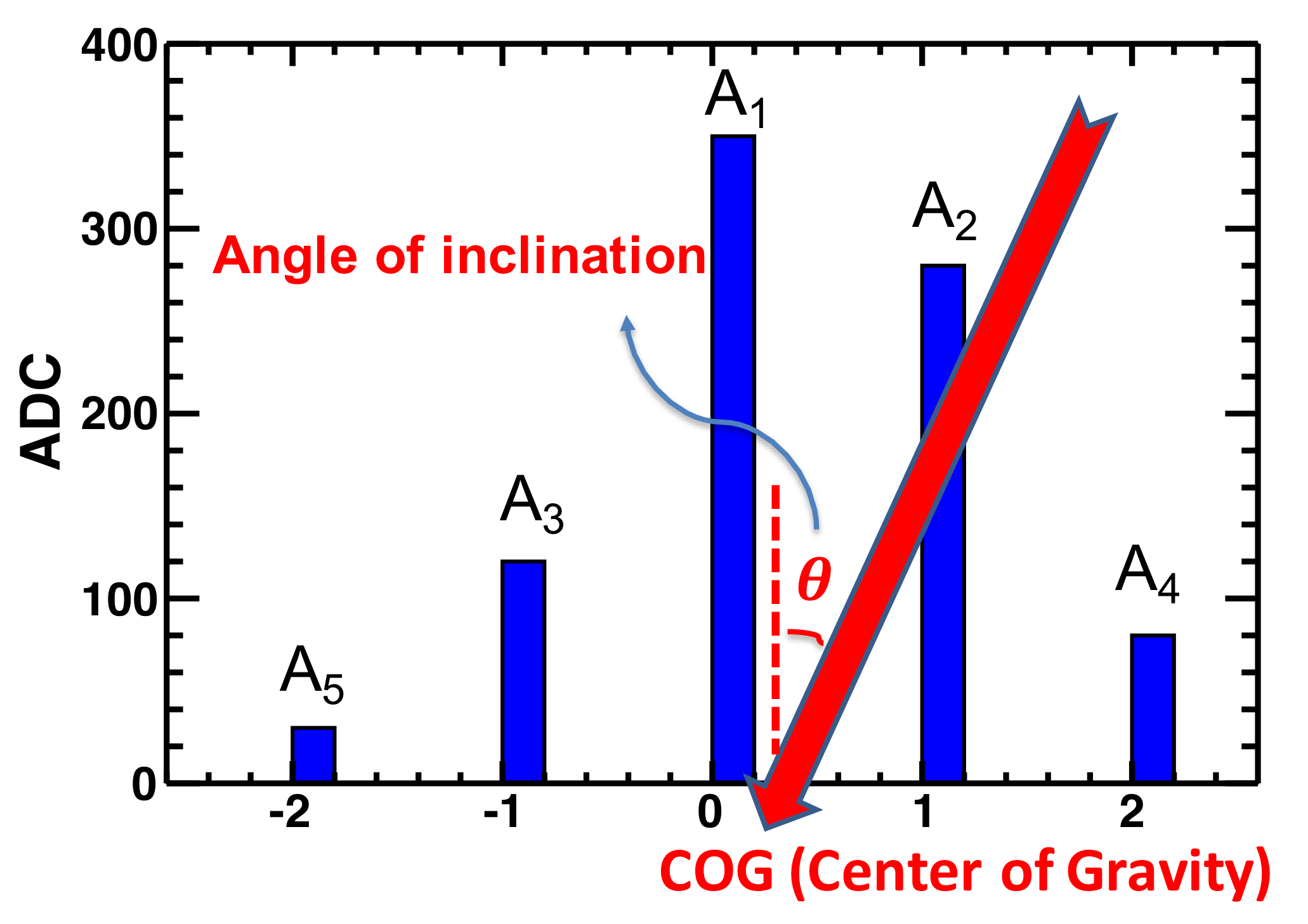
The energy loss deposition is collected by several strips on both sides and the relative signal on one side is related to the transverse distance between the strip and the location where the particle crosses the silicon, as shown in Figure 2. The strip with the highest amplitude (that is, the strip nearest to the crossing point) is called the seed strip or A1, the next highest adjacent strip A2, the other adjacent strip A3, etc.
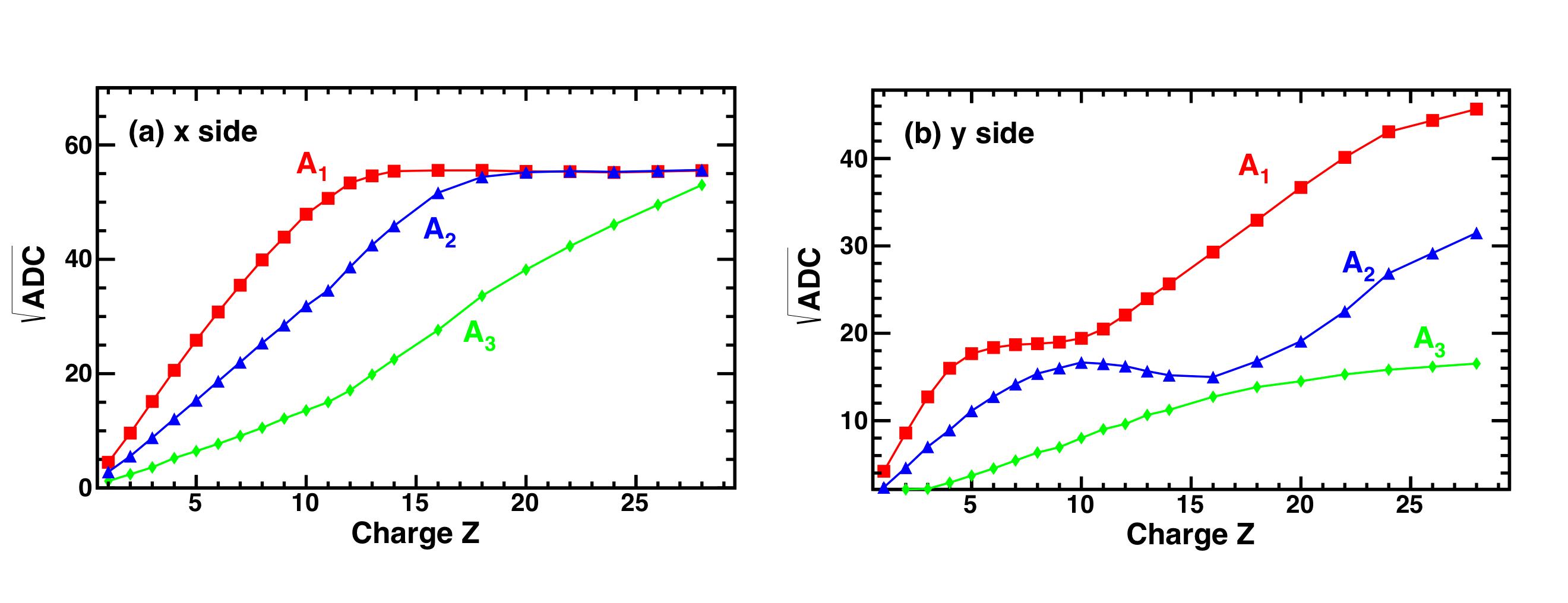
Previously, the charge measurement was taken as the square root of the sum of the charges measured on all strips. However, the x- and y-strips show very different non-linear response for high $Z$, as shown in Figure 3. This affects the accuracy of charge determination at high $Z$.
Optimal charge measurement requires several further corrections. For illustration, we show the two most important examples. The first one is equalization of the 196608 individual pulse heights of the tracker. The readout of the tracker strips is performed by 3072 multiplexers each connected to an individual amplifier, which reads out a group of 64 adjacent strips. Each amplifier has its own gain and calibration. This effect is presented in Figure 4.
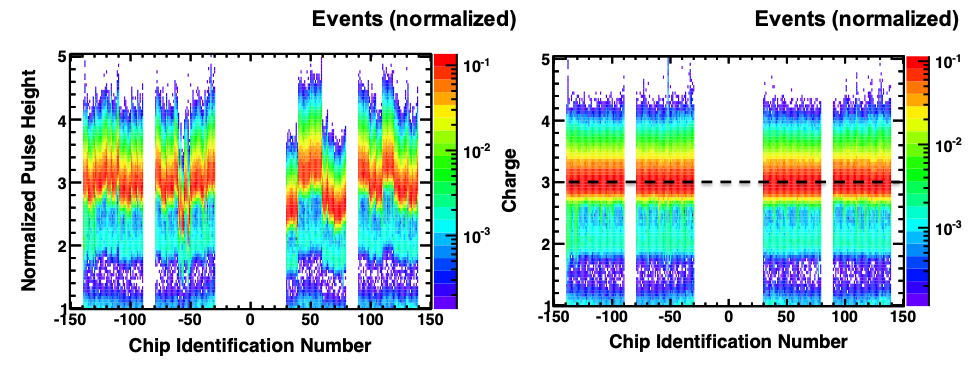
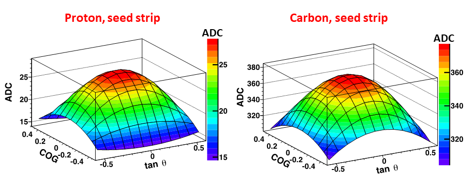
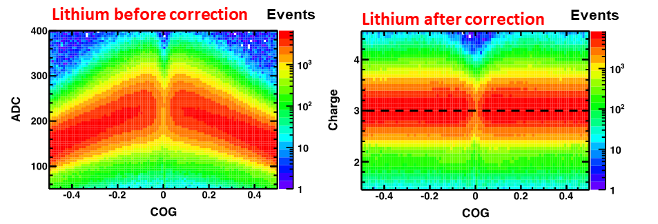
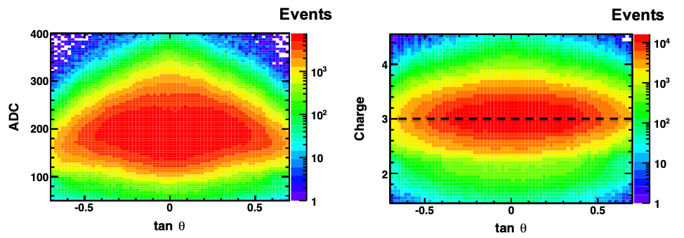
The second correction is due to the location of the center of gravity (COG) and the angle of incidence θ, both of which determine the amount of charge deposited and its relative distribution between strips as illustrated in Figure 2. To account for this effect, a correction is applied using pulse height distributions constructed for each $|Z|$ based on the distance from the COG in “strip” units, and the tangent of the angle of incidence ($\tan \theta$). Figure 5 shows the pulse height distributions as a function of COG and $\tan \theta$ for the seed strips for protons and carbon nuclei before the correction. The correction function is defined such that after correction the pulse height distributions are uniform in COG and $\tan \theta$. The improvement of the measured charge for lithium before and after this correction is shown in Figures 6 and 7.
After all the corrections (see Figures 4, 6, and 7), the individual strips for both x- and y- sides are used for the charge determination. The final charge is obtained by combining the x-side and the y-side measurements.
Of particular importance, with this new method we were able to improve the tracker charge resolution for $Z>10$ nuclei by a factor of two or more. For example, the combined charge resolution for silicon ($Z=14$) of tracker layers L2-L8 is 0.14, as shown in Figure 8 compared to 0.28 for the old method. This enables us to perform the precision measurement of all nuclei fluxes up to and beyond nickel ($Z=28$).
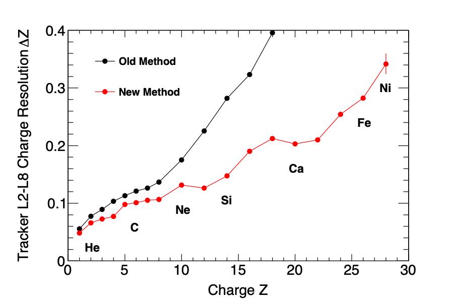
Figure 9 shows the comparison of the charge determination by the Time of Flight counters and the tracker (a) before and (b) after implementation of the new charge measurement technique. The improvement in the charge identification is clearly seen.